2  Finite Differences

Assume the general Poisson equation \[-\div(a\grad u)=f\]

with some conductivity \(a\), a source term \(f\) and the potential \(u\). This can be an electric potential with \(a=\sigma\), the hydraulic head with hydraulic conductivity \(k\), the temperature with the thermal conductivity or the gravity potential with \(a=1\). Note that we are using the form with the leading minus. First, \(-\grad u\) is typically the field (e.g. electric) and \(a\grad u\) is usually the flow (e.g. streaming velocity or current density) towards decreasing potential.

Neglecting \(a\) for a moment, the left-hand side is the second derivative, i.e. a curvature. A positive source field \(f\) leads to a negative curvature, i.e. a decreasing slope of the potential curve. This is a maximum of the potential caused by the source, e.g., an increased temperature for a heat source.

2.1 FD Approximation

Approximate derivative operators by differences

\[ \pdv{u}{x}\approx\frac{\Delta u}{\Delta x} \]

and solution \(u\) by finite values \(u_i\) at points \(x_i\), e.g. \[ \dv*{u}{x}_{2.5} := (u_3-u_2) / (x_3-x_2) \]

\[\pdv[2]{u_3}{x}\approx \frac{\dv*{u}{x}_{3.5}-\dv*{u}{x}_{2.5}}{(x_4-x_2)/2} = \frac{(u_4-u_3)/(x_4-x_3)-(u_3-u_2)/(x_3-x_2)}{(x_4-x_2)/2} \]

2.1.1 Difference stencil

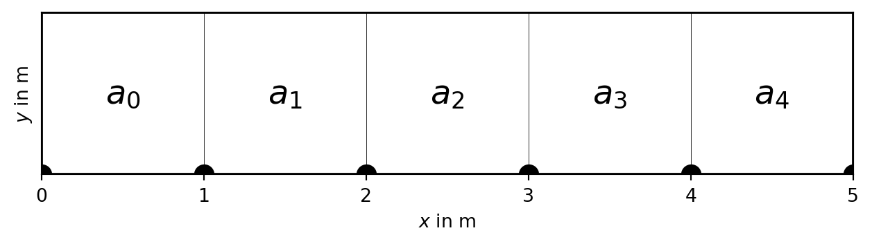
Assumption: equidistant discretization \(\Delta x\), conductivity 1

1st derivative: \([-1, +1] / dx\), 2nd derivative \([+1, -2, +1] / dx^2\)

Matrix-Vector product \(\vb{A}\cdot\vb{u}=\vb{f}\) with

\[ \vb{A} = \frac{1}{\Delta x} \begin{bmatrix} -1 & +2 & -1 & 0 & \ldots & & \\ 0 & -1 & +2 & -1 & 0 & \ldots & \\ \vdots & \vdots & \vdots & \ddots & \vdots & \\ \ldots & \ldots & 0 & -1 & +2 & -1 \end{bmatrix} \]

This is illustrated by the Finite Difference stencil (Figure 2.1): Every point, e.g. the red point, is constructed by using its neighbors.

Figure 2.1: 1D Finite-Difference stencil

2.2 FDM on the general Poisson equation

Assume the Poisson equation \[\div(a\grad u)=f\] with a conductivity term \(a\)

\[ \pdv{(a \pdv*{u}{z})}{z} = a\pdv[2]{u}{z} + \pdv{a}{z} \pdv{u}{z} \]

2.3 Boundary conditions

Dirichlet conditions: \(u_0=u_B\) (homogeneous if 0)

Neumann conditions (homogeneous if 0) \[ \pdv*{u}{x}_0=g_B \]

Mixed boundary conditions \(u_0+\alpha du_0/dx=\gamma\)

2.3.1 Dirichlet boundary conditions

Assume the dirichlet condition on the upper boundary \[u_0 = u_B \tag{2.1}\] fixes the potential to a specific value \(u_B\). #### Implementation 1 : explicit (2.1) can be directly added as an equation in the matrix and the right-hand-side:

\[ \begin{bmatrix} +1 & 0 & 0 & \ldots & & \\ -1 & +2 & -1 & 0 & \ldots & \\ \vdots & \vdots & \ddots & \vdots & \\ \ldots & \ldots & 0 & -1 & +2 & -1 \end{bmatrix} \cdot\vb{u} = \begin{bmatrix} u_B\\ f_1 \\ \vdots \\ f_N \end{bmatrix} \]

2.3.1.1 Implementation 2: Node removal

The Dirichlet condition (2.1) is directly inserted into the second equation \(-u_B + 2 u_1 - u_2 = f_1\) and the first equation is omitted

\[ \begin{bmatrix} +2 & -1 & 0 & \ldots & & \\ -1 & +2 & -1 & 0 & \ldots & \\ \vdots & \vdots & \ddots & \vdots & \\ \ldots & 0 & -1 & +2 & -1 \end{bmatrix} \cdot\vb{u} = \begin{bmatrix} f_1 + u_B\\ f_2 \\ \vdots \\ f_N \end{bmatrix} \]

Consequently, the first column is removed and the first equation is the sum of the preceding two other equations.

2.3.2 Neumann BC

The Neumann boundary condition \[ u_1 - u_0 = g_B \tag{2.2}\] fixes the gradient of the potential at the left end.

2.3.2.1 Implementation 1: explicit

The equation (2.2) replaces the first equation \[ \begin{bmatrix} -1 & +1 & 0 & \ldots & & \\ -1 & +2 & -1 & 0 & \ldots & \\ \vdots & \vdots & \vdots & \ddots & \vdots \\ \ldots & \ldots & -1 & +2 & -1 \end{bmatrix} \cdot\vb{u} = \begin{bmatrix} g_B\\ f_1 \\ \vdots \\ f_N \end{bmatrix} \] Note that this would result in an unsymmetric matrix for the left boundary, but in a symmetric matrix for the right boundary. Therefore we better use the outward normal direction \[ u_0 - u_1 = g_B \tag{2.3}\] leading to the symmetric matrix \[ \begin{bmatrix} +1 & -1 & 0 & \ldots & & \\ -1 & +2 & -1 & 0 & \ldots & \\ \vdots & \vdots & \vdots & \ddots & \vdots \\ \ldots & \ldots & -1 & +2 & -1 \end{bmatrix} \cdot\vb{u} = \begin{bmatrix} g_B\\ f_1 \\ \vdots \\ f_N \end{bmatrix} \]

2.3.3 Implementation 2: node removal

The equation (2.3) is directly inserted into the second equation \[-u_0 +2 u_1-u_2 = f_1\] This leads to \[u_2-u_1=f_1+g_B \] and thus to the matrix \[ \begin{bmatrix} +1 & -1 & 0 & \ldots & & \\ -1 & +2 & -1 & 0 & \ldots & \\ \vdots & \vdots & \ddots & \vdots & \\ \ldots & 0 & -1 & +2 & -1 \end{bmatrix} \cdot\vb{u} = \begin{bmatrix} f_1 + g_B\\ f_2 \\ \vdots \\ f_N \end{bmatrix} \]

2.4 The general case

\(\Delta x \ne 1\) & \(a \ne 1\) \(\Rightarrow\) \(a \pdv{u}{x} \approx a_i\frac{u_{i+1}-u_i}{x_{i+1}-x_i}\)

\(\dv{x}(a \pdv{u}{x}) \approx (a_i\frac{u_{i+1}-u_i}{x_{i+1}-x_i} - a_{i-1}\frac{u_{i}-u_{i-1}}{x_{i}-x_{i-1}}) / (x_{i+1}-x_{i-1}) \cdot 2\)

\[ A_{i, i-1} = a_{i-1} / (x_{i}-x_{i-1}) / (x_{i+1}-x_{i-1}) \cdot 2 \]

2.4.1 The coupling coefficients

\[ A_{i,i-1} = C_i^{left} = a_{i-1} / (x_{i}-x_{i-1}) / (x_{i+1}-x_{i-1}) \cdot 2 \]

\[ A_{i,i+1} = C_i^{right} = a_i / (x_{i+1}-x_{i}) / (x_{i+1}-x_{i-1}) \cdot 2 \]

\[ \begin{bmatrix} +1 & 0 & 0 & \ldots & & \\ C_1^L & -(C_1^L+C_1^R) & C_1^R & 0 & \ldots & \\ \vdots & \vdots & \ddots & \vdots & \\ \ldots & \ldots & 0 & C_N^L & -(C_N^L+C_N^R) & C_N^R \\ \ldots & \ldots & & 0 & -1 & +1 \end{bmatrix} \cdot\vb{u} = \begin{bmatrix} u_B\\ f_1 \\ \vdots \\ f_N \\ g_B \Delta x_N \end{bmatrix} \]

2.4.2 Symmetry

\[ A_{i+1,i} = C_{i+1}^{left} = a_i / (x_{i+1}-x_{i}) / (x_{i+2}-x_{i}) \cdot 2 \]

\[ A_{i,i+1} = C_i^{right} = a_i / (x_{i+1}-x_{i}) / (x_{i+1}-x_{i-1}) \cdot 2 \]

only symmetric if \(\Delta x\) is constant around \(x_i\), better take \(a_i/(\Delta x_i)^2\)

\[ A_{i,i-1} = C_i^{left} = a_{i-1} / (x_{i}-x_{i-1})^2 \]

\[ A_{i,i+1} = C_i^{right} = a_i / (x_{i+1}-x_{i})^2 \]

\(\Rightarrow\) inaccuracies expected for non-equidistant discretization

2.4.3 A closer look at the Dirichlet boundary

\[ \begin{bmatrix} +1 & 0 & 0 & \ldots & & \\ C_1^L & -(C_1^L+C_1^R) & C_1^R & 0 & \ldots & \end{bmatrix} \begin{bmatrix} u_B\\ f_1 \end{bmatrix}\]

1. \(C\) can be differently scaled from 1 \(\Rightarrow\) multiply with \(C_i^L\)
2. Matrix is non-symmetric

\[ \begin{bmatrix} C_1^L & 0 & 0 & \ldots & & \\ C_1^L & -(C_1^L+C_1^R) & C_1^R & 0 & \ldots & \end{bmatrix} \begin{bmatrix} u_B C_i^L\\ f_1 \end{bmatrix} \]

2.4.4 A closer look at the Neumann boundary

\[ \begin{bmatrix} \ldots & \ldots & 0 & C_N^L & -(C_N^L+C_N^R) & C_N^R \\ \ldots & \ldots & & 0 & -1 & +1 \end{bmatrix} \cdot\vb{u} = \begin{bmatrix} f_N \\ g_B \Delta x_N \end{bmatrix} \]

1. \(C\) can be differently scaled from 1 \(\Rightarrow\) multiply with \(C_N^R\)
2. Matrix is non-symmetric \(\Rightarrow\) multiply with -1

\[ \begin{bmatrix} \ldots & \ldots & 0 & C_N^L & -(C_N^L+C_N^R) & C_N^R \\ \ldots & \ldots & & 0 & C_N^R & -C_N^R \end{bmatrix} \cdot\vb{u} = \begin{bmatrix} f_N \\ -g_B \Delta x_N C_N^R \end{bmatrix} \]

2.4.5 Accuracy

How can we prove the accuracy of our solution?

• compare with analytical solutions
• single (Point) \(f\) lead to piece-wise linear \(u\) (correct)
• what about continuous source terms?
  (e.g. radioactive elements in the Earth’s crust)

2.4.6 Analytical solution

\(a\)=1, \(f(x)\)=1 \(\Rightarrow\) double integration \(\Rightarrow\) quadratic function

\[u(x) = C_0 + C_1 x -1/2 x^2 \]

Left BC	Right BC	\(C_0\)	\(C_1\)
Dirichlet	Dirichlet	\(u_L\)	\(L/2 + (u_R-u_L)/ L\)
Dirichlet	Neumann	\(u_L\)	\(g_R + L\)
Neumann	Dirichlet	\(u_R - g_L L + L^2/2\)	\(g_L\)

with \(L=(x_N-x_0)\)

2.4.7 Next spatial dimension

If we go from 1D to 2D conditions, we have conductivities between each four nodes (Figure 2.2). The red point is constructed by its four neighbors to the left and right, and to the top and bottom.

Figure 2.2: Simple 2D conductivity grid with FD stencil

For introducing the conductivity into the coupling coefficient, there are always two values adjacent to the connecting edge.

\[ C_{i,j}^{right} = a_{i,j-1/2} / (x_{i+1}-x_{i})^2 \]

\(a_{i,j-1/2}=(a_{i,j-1}+a_{i,j})/2\) ?

harmonic, geometric? weighting?

\(a_{i,j-1/2}=\frac{a_{i,j-1}\Delta y_{j-1}+a_{i,j}\Delta y_{j}}{y_j+1-y_{j-1}}\)?

2.5 Parabolic PDEs

2.5.1 Heat transfer in 1D

\[ \pdv{T}{t} - a \pdv[2]{T}{z} = 0 \]

with the periodic boundary conditions:

• \(T(z=0,t)=T_0 + \Delta T \sin \omega t\) (daily/yearly cycle)
• \(\pdv{T}{z}(z=z_1) = 0\) (no change at depth)

and the initial condition \(T(z, t=0)=\sin \pi z\) has the analytical solution \[ T(z, t) = \Delta T e^{-\pi^2 t} \sin \pi z \]

2.5.2 Periodic boundary conditions

\[ \pdv{T}{t} - \div (a\grad{T}) = \div q_s \]

• \(a=\frac{k}{\rho c_p}\) [m²/s] thermal diffusivity - measure of heat transfer
• \(k\) [W/m/K] thermal conductivity - measure of temperature transfer
• \(c_p\) [J/kg/K] - heat capacity - measure of heat storage per mass
• \(\rho\) (kg/m³) density

Water \(k\)=0.6 W/m/K, \(\rho\)=1000 kg/m³, \(c\)=4180 J/kg/K \(\Rightarrow\) \(a\)=1.43e-7 m²/s

Upper boundary: daily/yearly variation

\[ T_0(t) = T_m + \Delta T \sin \omega t \]

\(T_m\) mean temperature (e.g. 12°C), \(\Delta T\) variation, e.g. 8°C

\(\omega=2\pi/t_P\) daily (\(T_d\)=3600*24s) or yearly (\(T_y=365 T_d\)) cycle ::: ::: {.column}

day = 3600 * 24
T0, dT = 12, 8
t = np.arange(100) / 50 * day
T = T0+dT*np.sin(t/day*2*np.pi)
plt.plot(t/day*24, T)
plt.xlabel("t (h)")
plt.ylabel("T (°C)")
plt.grid()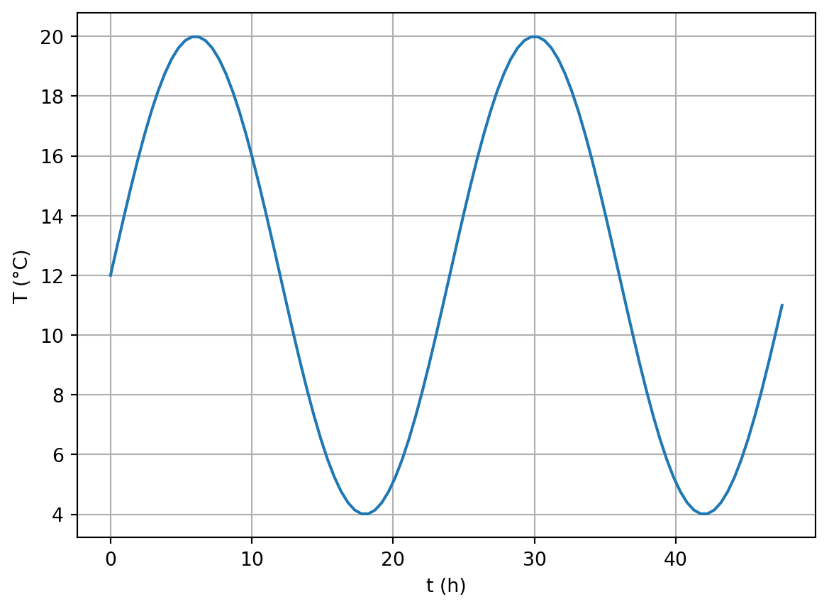

2.5.3 Separation of variables

\[ \pdv{T}{t} = a\pdv[2]{T}{z} \]

\(T(t, z)/\Delta T - T_0 = \theta(t) Z(z)\)

\[ Z \pdv{\theta}{t} = a \theta \pdv[2]{Z}{z} \]

\[ \frac1\theta \pdv{\theta}{t} = C = a \frac{1}{Z}\pdv[2]{Z}{z} \]

2.5.4 Solution

regarding the BC \(e^{\imath\omega t}\) leads to \(C=\imath\omega\) and thus \(\theta=\theta_0 e^{\imath\omega t}\)

\[ \pdv[2]{Z}{z} - \imath \frac{\omega}{a} Z = \pdv[2]{Z}{z} + n^2 Z = 0 \]

Helmholtz equation with solution \(Z=Z_0 e^{\imath n z}\) (\(n^2=\imath\omega/a\))

\[ Z=Z_0 e^{\imath n z} = Z_0 e^{\sqrt{\imath\omega/a}z} = Z_0 e^{\sqrt{\omega/2a}(1+\imath)z} \]

\[ T(t, z)/\Delta T + T_0 = Z(z)\theta(t)= Z_0\theta_0 e^{-\sqrt{\omega/2a}z} e^{i(\omega t-\sqrt{\omega/2a}z)} \]

2.5.5 Interpretation

replacing the term \(\sqrt{2a/\omega}=\sqrt{a t_P/\pi}=d\) leads to

\[ T(z, t) = T_0 + \Delta T e^{-z/d} \sin(\omega t - z/d) \]

• exponential damping of the temperature variation with decay depth \(d\)
• phase lag \(z/d\) increases with depth, \(z_\pi=\sqrt{2 a/\omega}\pi=\sqrt{a t_P \pi}\)

1. Daily cycle: decay depth \(d\)=6cm, minimum depth=20cm
2. Yearly cycle: decay depth \(d\)=1.2m, minimum depth=4m

2.5.6 Depth profiles

a = 1.5e-7
year = day*365
d = sqrt(a*year/pi)
t = np.arange(0, 1, 0.1) * year
z = np.arange(0, 6, 0.1)
fig, ax = plt.subplots()
for ti in t:
    Tz = np.exp(-z/d)*np.sin(ti*2*pi/year-
                             z/d) * dT + T0
    ax.plot(Tz, z, label="t={:.1f}".format(
        ti/year))

ax.invert_yaxis()
ax.legend()
ax.grid()

2.5.7 Temporal behaviour

t = np.arange(0, 1.01, 0.01) * year
z = np.arange(0, 3, 0.4)
fig, ax = plt.subplots()
for zi in z:
    Tt = np.exp(-zi/d)*np.sin(t*2*pi/year-
                              zi/d) * dT + T0
    ax.plot(t/year*12, Tt, label=f"z={zi:.1f}")

ax.set_xlim(0, 12)
ax.set_xlabel("t (months)")
ax.set_ylabel("T (°C)")
ax.legend()
ax.grid()

2.5.8 Explicit method

\[ \pdv{T}{t} - a \pdv[2]{T}{z} = 0 \]

Solve Poisson equation \(\div(a\grad u)=f\)

for every time step \(i\) (using FDM, FEM, FVM etc.)

Finite-difference step in time: update field by \[ T_{i+1} = T_i + a \pdv[2]{u}{z} \cdot \Delta t\]

Forward difference stencil

2.5.9 Implicit (Euler) method

\[ \pdv{T}{t}^n \approx \frac{T^{n+1}-T^n}{\Delta t} = a \pdv[2]{T}{z} ^{n+1} \]

Forward difference stencil

2.5.10 Mixed - Crank-Nicholson method

\[ \pdv{T}{t}^n \approx \frac{T^{n+1}-T^n}{\Delta t} = \frac12 a \pdv[2]{T}{z} ^n + \frac12 a \pdv[2]{T}{z} ^{n+1} \]

Mixed (balanced) difference stencil

2.6 Hyberbolic equations

Acoustic wave equation in 1D \[ \pdv[2]{u}{t} - c^2\pdv[2]{u}{x} = 0 \]

\(u\)..pressure/velocity/displacement, \(c\)..velocity

Damped (mixed parabolic-hyperbolic) wave equation \[ \pdv[2]{u}{t} - a\pdv{u}{t} - c^2\pdv[2]{u}{x} = 0 \]

2.6.1 Discretization

\[ \pdv[2]{u}{t}^{n} \approx \frac{u^{n+1}-u^n}{\Delta t} - \frac{u^{n}-u^{n-1}}{\Delta t} \]

\[ = \frac{u^{n+1}+u^{n-1}-2 u^n}{\Delta t^2} = c^2\pdv[2]{u}{x}^n \]

\[ u^{n+1} = c^2 \Delta t^2 \pdv[2]{u}{x}^{n} + 2 u^n - u^{n-1} \]

\[ \vb M \vb u^{n+1} = (\vb A + 2\vb M) \vb u^n - \vb M \vb u^{n-1} \]

Second derivative

2.6.2 Example: velocity distribution

import numpy as np
import matplotlib.pyplot as plt
x=np.arange(0, 600.01, 0.5)
c = 1.0*np.ones_like(x) # velocity in m/s
c[100:300] = 1 + np.arange(0,0.5,0.0025) 
c[900:1100] = 0.5  # low velocity zone

# Plot velocity distribution.
plt.plot(x,c,'k')
plt.xlabel('x [m]')
plt.ylabel('c [m/s]')
plt.grid()

2.6.3 Initial displacement

Derivative of Gaussian (Ricker wavelet)

l=5.0

# Initial displacement field [m].
u=(x-300.0)*np.exp(-(x-300.0)**2/l**2) 
# Plot initial displacement field.
plt.plot(x,u,'k')
plt.xlabel('x [m]')
plt.ylabel('u [m]')
plt.title('initial displacement field')
plt.show()

2.6.4 Time propagation

u_last=u
dt = 0.5
ddu = np.zeros_like(u)
dx = np.diff(x)
for i in range(100):
    dudx = np.diff(u)/dx
    ddu[1:-1] = np.diff(dudx)/dx[:-1]
    u_next = 2*u-u_last+ddu*c**2 * dt**2 
    u_last = u
    u = u_next
  
plt.plot(x,u,'k')