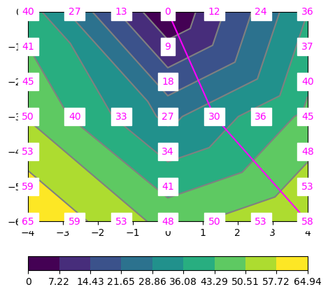
Show the code
import pygimliThe physical fields are governed by partial differential equations with differential operators in space and time There are single derivative in space \(\pdv{x}\) or time \(\pdv{t}\). All derivatives into all spatial dimensions are subsumed in the nabla operator \(\grad=(\pdv x, \pdv y, \pdv z)^T\). The (negative) gradient of a potential is the corresponding vector field with directions perpendicular to the isosurfaces into the direction of decreasing potential.
The divergence applies the nabla operator to a vectorial field by the dot product: \[\div \vb F = \pdv{F_x}{x} + \pdv{F_y}{y} + \pdv{F_z}{z}\] The divergence of a field describes the source strength using Gauss’ law.
Gauss’ law:
what’s in (volume) comes out (surface) \[\int_V \div\vb F\ dV = \iint_S \vb F \vdot \vb n\ dS\]
The curl (rotation) operator occurs particularly in electromagnetic problems, where magnetic fields are caused by (conduction or displacement) currents and electric fields infer changes in the magnetic field. It is described by the cross-product between nabla operator and the field \[\curl \vb F = (\pdv{F_z}{y}-\pdv{F_y}{z}, \pdv{F_x}{z}-\pdv{F_z}{x}, \pdv{F_y}{x}-\pdv{F_x}{y})^T\]
Stokes law:
what goes around comes around \[\int_S \curl \vb F \vdot \vb dS = \iint_S \vb F \vdot \vb dl\]
There are two laws concerning curl fields:
fdgdfhrfgh
Mostly: solution of partial differential equations (PDEs) for either scalar (potentials) or vectorial (fields) quantities.
(\(u\)-function, \(f\)-source, \(a\)/\(c\)-parameter):
potential field \(u\) generates field \(\vec{F}=-\nabla u\)
causes some flow \(\vec{j}=a \vec{F}\)
\(a\) is some sort of conductivity (electric, hydraulic, thermal)
continuity of flow: divergence of total current \(\vb j + \vb j_s\) is zero
\[ \div (a \nabla u) = - \div \vb j_s \]
sought: Temperature \(T\) as a function of space and time
heat flux density \(\vb q = \lambda\grad T\)
\(q\) in W/m², \(\lambda\) - heat conductivity/diffusivity in W/(m.K)
Fourier’s law: \(\pdv{T}{t} - a \nabla^2 T = s\) (\(s\) - heat source)
temperature conduction \(a=\frac{\lambda}{\rho c}\) (\(\rho\) - density, \(c\) - heat capacity)
volumetric flow rate \(Q\) caused by gradient of pressure \(p\)
\[ Q = \frac{k A}{\mu L} \Delta p \]
\[\vb q = -\frac{k}{\mu} \nabla p \]
\[\div\vb q = -\div (k/\mu \grad p) = 0\]
\[ \mu \nabla^2 \vb v - \grad p + f = 0 \]
\[\div\vb v = 0 \]
e.g. from Fourier assumption \(u=u_0 e^{\imath\omega t}\)
\[ \div (a\grad u) + k^2 u = f \]
\[ \Rightarrow \vb A + \vb M = \vb b \]
\[ \nabla^2 u + k^2 u = f \]
results from wavenumber decomposition of diffusion or wave equations
approach: \(\vb F = \vb{F_0}e^{\imath\omega t} \quad\Rightarrow\quad \pdv{\vb F}{t}=\imath\omega\vb F \quad\Rightarrow\quad \pdv[2]{\vb F}{t}=-\omega^2\vb F\)
\[ \nabla^2 \vb F - a \nabla_t \vb F - c^2 \nabla^2_t \vb F = 0 \]
\[ \Rightarrow \nabla^2\vb F - a\imath\omega\vb F + c^2 \omega^2\vb F = 0 \]
Describes first-arrival times \(t\) as a function of velocity (\(v\)) or slowness (\(s\))
\[ |\grad t| = s = 1/v \]

Acoustic wave equation in 1D \[ \pdv[2]{u}{t} - c^2\pdv[2]{u}{x} = 0 \]
\(u\)..pressure/velocity/displacement, \(c\)..velocity
Damped (mixed parabolic-hyperbolic) wave equation \[ \pdv[2]{u}{t} - a\pdv{u}{t} - c^2\pdv[2]{u}{x} = 0 \]
import pygimli